Problem: 

"Bayesian Thinking" -> "Programming Probability Distributions" -> "Visualizing a Piece-Wise Continuous Probability Distribution"

Write a function that, given a list of x-axis intervals, relative probabilities and a total probability, calculates the height of each bar. Remember that the sum of the area for all bars should be the total probability.

Here is an example input and output:

• a vehicle accident is 5 times more likely from 5am to 10am versus midnight to 5am.
• a vehicle accident is 3 times more likely from 10am to 4pm versus midnight to 5am.
• a vehicle accident is 6 times more likely from 4pm to 9pm versus midnight to 5am.
• a vehicle accident is 1/2 as likely from 9pm to midnight versus midnight to 5am.
• The probability of getting in an accident on any given day is .05

The inputs would look like this.

For the hours, you can use 24 hour time
hour_intervals = [0, 5, 10, 16, 21, 24]
relative_probabilities = [1, 5, 3, 6, 0.5],
total_probability = 0.05

The output would be the height of each bar:
[0.0006451612903225806, 0.0032258064516129032, 0.0016129032258064516, 0.003870967741935484, 0.0005376344086021505]

At the end of the exercise, your visualization should look like this:

Hints

• Summing the area of all the bars equals the total probability, which in this case is 0.05.
• The relative probabilities and total probability can be used to find the exact area of each bar. If the area of the first bar is A, then the area of the second bar is 5A, the third bar is 3A, etc.
• Once you know the area of each bar, you can divide each area by its width to calculate the bar height.

I was stuck as I could not understand, why the area under distribution should be total probability which is 0.05, which was against the notion taught earlier that area under density function should be 1.

Direct answer: It is because, its not yet normalized distribution. Or in other words, its just joint probability we calculated instead of posterior probability. Let us see how.

We will first approach conceptually and solve why total area is total probability 0.05 and then go to programming. We will also use an alternate approach in our logic and compare our results with what Udacity arrived at.

Section 1: Why the heck the total area is not 1 but total probability.

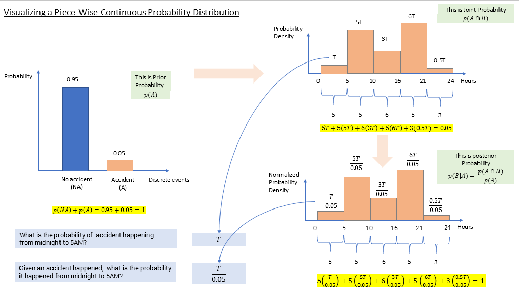
It is given that at any day, the probability of accident happening is 0.05. Below would be its probability distribution. This is discreet, and hence y-axis is probability, and they all add up to 1, of course. This is like a prior probability we have more evidence next to come. All good.

Next evidence is that, when an accident happens, there are different probabilities for different time zones.  This is a joint probability. An accident happening and its happening in a particular time slot.

We will come to the equation below chart in Figure 2 shortly. Note the first probability is taken as T because we are given relative probabilities, relative to that first time zone. For eg, accident between 5 to 10 AM is 5 times more likely than from midnight to 5 AM. This is also a piece wise continuous distribution because, x-axis is in hours which is continuous, but instead of a curve on y, we have different uniform distribution in different time slots. So its uniform over a time slot and has discontinuity when time slot changes, thus piece wise. (Realistically this could have been a curve, and then our area calculation would  be complicated)

Now total area which is crux of the issue.

Probability of accident in a day is 0.05.

Thus probability of accident in any time slot over the day is 0.05. If nth time slot event is named, say Tn, then

$p(T_{1} \cup T_{2}... \cup T_{n})=0.05$

Since all are mutually exclusive, independent.. (we are not considering 2 or more accidents in a row in this problem)

$p(T_{1}) + p(T_{2})... + p(T_{n})=0.05$

For each time slot, probability can be calculated from distribution as its uniform distribution area. For eg for first time slot, its (5-0)*T = 5T. Thus,

5T+5(5T)+6(3T)+5(6T)+3(0.5T)=0.05(1)

Thus,

$\text {T} = \frac{0.05}{5+25+18+30+1.5}=\frac{0.05}{79.5} = 0.00062893081$(2)

Calculating further for each time slot, the height as multiple of T we saw in Figure 2, we could get, height array as,

{0.0006289308176101, 0.0031446540880505, 0.0018867924528303, 0.0037735849056606,0.00031446540880505}(3)

Hmm, this is different to an extent, the solution from Udacity.

{0.0006451612903225806, 0.0032258064516129032, 0.0016129032258064516, 0.003870967741935484, 0.0005376344086021505}(4)

Let us compare the accuracy of both results. Since the area of entire distribution should be 0.05, let us calculate these individual heights with their respective widths (time slots or intervals) and see which gives better results for the total area which should be 0.05.

Our accuracy:

0.0006289308176101 + 50.0031446540880505 + 60.0018867924528303 + 50.0037735849056606 + 30.00031446540880505 =0.04748427672956255

$\text {Accuracy}= \big(\frac{0.04748427672956255}{0.05})100 = 94.9685534591251 \%$

Udacity's accuracy:

0.0006451612903225806 + 50.0032258064516129032 + 60.0016129032258064516 + 50.003870967741935484 + 30.0005376344086021505 = =0.0474193548387096777

$\text {Accuracy}= \big(\frac{0.0474193548387096777}{0.05})100 = 94.8387096774193554 \%$

Its almost the same. In fact, ours is slightly better with 0.1 % more accuracy.

Thus let us stick with our concept unless proven wrong. (for eg, check last time slot. we got 0.00031446540880505 while Udacity has 0.0005376344086021505, which is a considerable difference).

Normalization:

We thus have derived "joint probability" distribution p(A ∩ B). What about posterior probability? For eg, given an accident happened, what is the probability it happened from midnight to 5 AM?

We now know,

$\text {p(A) = probability of accident in a day = 0.05}\ \text {p(A} \cap \text{B) = probability of accident in a day and in a particular time slot}$

From Bayes theorem,

$\text {p(B} \mid \text{A)} = \frac{\text{p(A} \cap \text{B)}}{\text p(A)}$

The graph and derivation would be something like below, left to readers to try out. Just divide the heights by 0.05, to get total area as 1 as illustrated below.

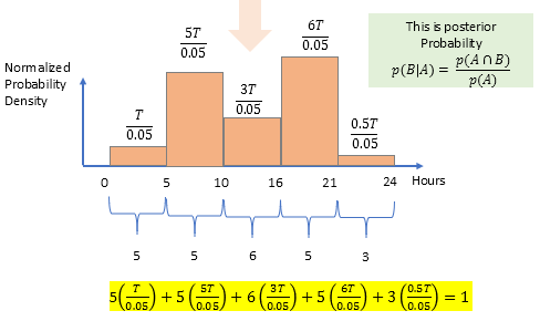
Summarizing visually,

The result of normalized distribution would be

{0.012578616352202, 0.06289308176101, 0.037735849056606, 0.075471698113212, 0.006289308176101}

Note the probabilities are higher compared to our previous joint probability case. This is understandable right? Given that an accident already occurred, now your perceived probabilities on which slot would it have occurred would be more.

Program is just direct implementation of our logic, with slight adaptation to handle the lists. Recall the inputs provided: intervals list, relative probabilities list, total probability.

First we create another list which only contains intervals from the intervals list (in fact, incoming interval list is kind of misnomer). Then we could multiply that with relative probabilities along with T factor, as their sum should equal to 0.05. This will allow us to derive T eventually. Using T on relative probabilities we could then generate heights array. Here is the visualization with an example.

Implementing our logic in python:

import numpy as np
def bar_heights(intervals, relative_probabilities, total_probability):

delta_intervals = [intervals[i+1]-intervals[i] for i in range(len(intervals)-1)]
area = np.multiply(delta_intervals, relative_probabilities)
heights = [(total_probability/sum(area))*x for x in relative_probabilities]

return heights

print(bar_heights([0, 5, 10, 16, 21, 24], [1, 5, 3, 6, 0.5], 0.05))

Udacity's concept for comparision:

def bar_heights(intervals, probabilities, total_probability):

heights = []
total_relative_prob = sum(probabilities)
for i in range(0, len(probabilities)):
bar_area = (probabilities[i] / total_relative_prob) * total_probability
heights.append(bar_area / (intervals[i + 1] - intervals[i]))

return heights
print(bar_heights([0, 5, 10, 16, 21, 24], [1, 5, 3, 6, 0.5], 0.05))

I hope, my concept and code would also be acceptable as answer.